Although there is no Gantt chart tool in Microsoft Excel 2003, you can easily create your own from a horizontal bar chart, provided you know which options to select and deselect, and which settings to tweak. If you have not created a Gantt chart using Excel’s Chart Wizard before, create a basic chart first based on three tasks with different start dates and different duration times. Once you have gone through the process once, use this basic chart as a guide to create a Gantt chart based on your own data.
Creating the Spreadsheet
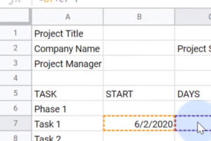
1.Launch Excel and open a new worksheet by pressing “Ctrl-N” on the keyboard. Note that the first column and first row should be reserved for titles only.
2.Type “Event” in cell A1, “Start Date” in cell B1, and “Days” in cell C1. Type “First Task” in cell A2, “Second Task” in cell A3 and “Third Task” in cell A4
3.Type “1-March-2012” in cell B2, “3-March-2012” in B3 and “10-March 2012” in cell B4. Type “5” in cell C2, “2” in C3 and “3” in C4. Note that this format shows that the first task begins March 1 and lasts five days. The second task begins March 3 and lasts two days. The third task begins March 10 and lasts three days.
Creating a Gantt Chart
1.Click cell “A1” and hold down the mouse button. Drag the mouse to cell “C4.” All of the populated cells are highlighted.
2.Click the “Insert” menu and select “Chart.” The Excel Chart Wizard opens. Select “Bar” from Chart Type menu, then click “Stacked Bar” from the Chart Sub-Type menu. Click “Next.”
3.Select “Columns” in Step 2 of the Chart Wizard. Click the “Series” tab. Note that there is only one series listed. Click the “Add” button beneath the Series section to add a second series.
4.Select the first series in the Series list by clicking it. In this example, this may be called the “Duration” series. This name is meaningless in making a Gantt Chart. Type “=Sheet1!$B$2:$B$4” in the Values field, which specifies cells B2 to B4 and represents the dates listed in the spreadsheet.
5.Click “Series 2” in the Series section. Type “=Sheet1!$C$2:$C$4” in the Values field, which specifies the duration data in the spreadsheet located in cells C2 to C4. The bottom two bars in the preview window should each be two colors. Click “Next.”
6.Click the “Legend” tab and deselect the “Show Legend” options. Click “Finish.” The chart is added to the spreadsheet. Move the chart if desired by clicking any empty area in the chart and dragging it. You can also resize it as needed by dragging its corners.
7.Double-click any number at the bottom of the chart. These numbers are the Value Axis. The Format Axis dialog box opens. Click the “Scale” tab. Type the minimum date on the spreadsheet (“1-March-2012” in the example in the Minimum text field. Type the maximum date (“13-March-2012”) in the Maximum field. Type “7” in the Major Unit field to specify one week. Type “1” in the Minor Unit field to specify one day. Click “OK.”
8.Double-click any of the tasks in the left side of the chart, which represent the Category Axis. Click the “Scale” tab. Select the “Categories in Reverse Order” and “Value (Y) Axis Crosses at Maximum Category” options. Click “OK.”
9.Double-click the left color of any of the bars in the chart. The Format Data Series dialog box opens. Click the “Patterns” tab. Set the “Border” and “Area” options to “None.” Click “OK.” The first half of each bar is now invisible, making the remaining bars appear staggered in their placement and completing the Gantt Chart.